A Primer on Spherical Harmonic Projections for Atomic Environments

• Spherical harmonics are the basis functions for signals on the sphere ($S^2$)
• Spherical harmonics are great for describing local atomic environments
• Many coefficients become zero for objects with symmetry
• Plotting the value of spherical harmonic coefficents are a quick way to see where zeros are occuring

The aim of this post is give some examples of spherical harmonic projections to play with to build intuition about why spherical harmonics are so helpful for describing atomic environments.

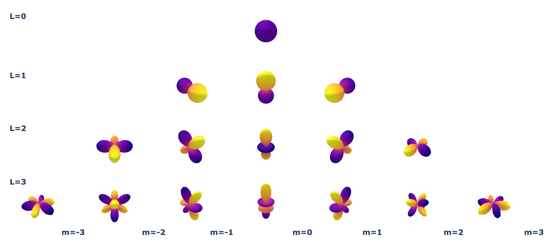
Spherical harmonics are the basis functions for signals on the sphere ($S^2$)

Below we'll plot the real spherical harmonics as 3D Surface plots where the magnitude of the signal is the radial distance of the point of the surface from the origin. In this plot, Yellow signifies positive values and Blue signifies negative values.

Spherical harmonics are great for describing local atomic environments

Why? Atoms don’t like to be too close to each other — they tend to spread themselves evenly across the sphere when coordinating a central atom. This means that we don’t need to go to high in spherical harmonic order to capture a local environment. We only need high L to differentiate between two points that are close together in angle.

To demonstrate this, we plot the spherical harmonic projection of two vectors with angle $\theta$ between them with $L_{max} = 4$. We will see that the needed $L$ to achieve a good angular resolution is $L \approx 2 \pi / \text{minimum angle}$.

As the minimum angle approaches zero $L \rightarrow \infty$, but practically, the angles between triplets of atoms rarely come close to this and $L_{max} = 6 - 10$ is often sufficient, especially when using radial basis functions (to account for radial degrees of freedom) with spherical harmonics describing the angular degrees of freedom.

Many coefficients become zero for objects with symmetry

Another time when we need higher L is when we have high symmetry. For example, you can’t represent n-fold symmetry with lower than L=n. In the example below, we'll see that high symmetry configurations like the vertices of a tetrahedron or octahedron.

Plotting the value of spherical harmonic coefficents are a quick way to see where zeros are occuring

Another way to examine this data is the plot the coefficients associated with each of the spherical harmonics. In this plot the y-axis indicates the different configurations and the x-axis indicates the L and m of each $(L_{max} + 1)^2$ coefficents. As we will see, many of these coefficients are zero, matching the lack of features for some of the plots above.